为什么要进行数据可视化?
1.相比于文字,将文字进行可视化可以让大脑能够同时处理更多的数据。例如,如果读到下面一段文字
3rd Street is to the north of 4th Street. Peach Avenue runs perpendicular to 3rd and 4th streets. On the southeast corner of 4th and Peach is a coffee shop. On the northwest corner of 3rd and Peach is a tea store.
How many streets does a person need to cross when walking from the coffee shop to the tea store?
如果用文字来表述这段信息会让很多不认路的人理解起来非常困难,但是如果直接给你下面一张图: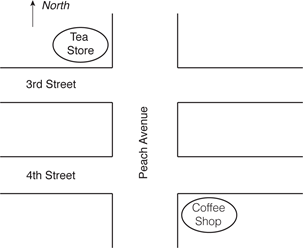
答案就一目了然了。
2.相较于文字,可视化能够使传递出的信息更加清晰,例如如果你读到下面一段话
The cross is above the rectangle. The triangle is next to the rectangle.
在文字中,这句话所反映出的信息就比较模棱两可:在矩形上面是十字形,三角形与矩形相邻。这个相邻就是一个模棱两可的解释,因为相邻既可以在左边,也可以在右边,前面或者后面。但是如果你用一幅图来表示这个信息的话,那么你就可以非常清楚地看清楚这三个图形的位置关系。
3.当我们将数据可视化的时候,可以看到一些用文字无法看到的信息。
例如下面的这个散点图: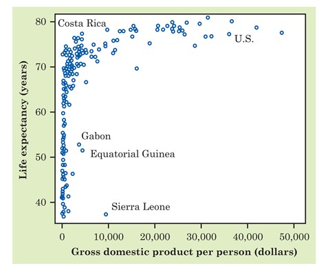
如果只用文字表示,那我只能看到一个个冷冰冰的数字,很难从数字中看到规律,但是如果利用散点图,我们可以清楚地看到这个些数据的变化趋势
图中的点代表全世界每一个提供数据的国家。横轴是对国家富裕程度的一种量度,即人均GDP,通常以美元为单位;纵轴是人的预期寿命。我们预计富裕国家的人应该寿命更长些。散点图的整体形态的确反映了这种情况,但两个变量间的关系表现为有趣的形状。当人均GDP增加时,起初预期寿命急速增加,但是后来呈平稳状态。像美国这样的富国的民众,并不比比较贫穷但非最贫穷国家的人预期寿命更长。有些国家,比如哥斯达黎加,其民众的预期寿命甚至超过美国。三个非洲国家是异常值,它们的民众预期寿命与邻国差不多,但人均GDP较高,它们分别是产油国赤道几内亚、加蓬,以及出产钻石的塞拉利昂。这可能是因为出口矿产的收入主要流入了少数人的腰包从而推高了人均GDP,但并没有对普通民众的收入或预期寿命产生多大的影响。换言之,人均GDP是一个平均数,我们知道收入的平均数可能远高于收入的中位数。
数据可视化的主流工具有哪些?
| Name | Open Source or Not | Free or not | Program or not |
|---|---|---|---|
| Tableau | No | Public edition – Free | No |
| D3.js | Yes | Yes | Yes |
| Power BI | No | No | No |
| R | Yes | Yes | Yes |
| Python | Yes | Yes | Yes |
| Matlab | No | No | Yes |
Tableau和Power BI是比较受欢迎的商业数据可视化工具,但是这两个都是付费的,作为穷科研民工不予考虑,D3.js是javascript的一个包,IT界用的比较多,Matlab是数据建模用的比较多在国科大的时候教生物统计的老师曾经跟我们一通安利)。Python虽然现在很受欢迎,但是我之前用过后觉得绘图方面还是不如R。R在科研界用的比较多,因此作为科研民工就遵循传统,也用R。
为什么要使用ggplot2?
用R进行数据可视化可以有多种选择,你可以用R的基础绘图系统,也可以使用其他的包,例如ggplot2、Lattice等等。最开始我是用的基础的R绘图系统,但是用起来很多时候比较蹩脚,后来开始尝试ggplot2,感觉ggplot2才是深得我心,当然,选择ggplot2的不止我一个人,作为科研民工,每一个选择都要有理有据,在ggplot2的github上有一个页面列出了为什么使用ggplot2的理由,这些理由是不同的人写的,因此很多观点都有重复,我个人将这些理由总结了下,可以归为四点,以下将分别说明。
1.良好的默认设置
相比于基础的R绘图系统,ggplot2默认的颜色设置和图形布局更为漂亮(尤其是图形布局),你不需要知道太多的主题设置方法也能画出漂亮的图,从这一点来说,ggplot2的下限比基础的R绘图系统更高(当然,上限我认为ggplot2比起基础的R绘图系统来说也更高),当然,我这么说很多习惯用R基础绘图的会不同意,口说无凭,直接举例子。
先说布局的问题,比如我现在想画一个直方图,这里R里面自带的mtcars数据举例,用基础的R绘图系统画出来的图是这样的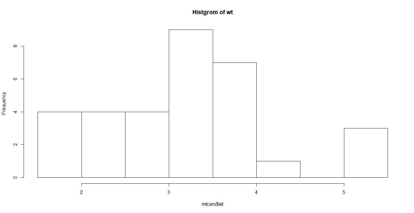
1
hist(mtcars$wt,main="Histgrom of wt")
用ggplot2画出来的是这样的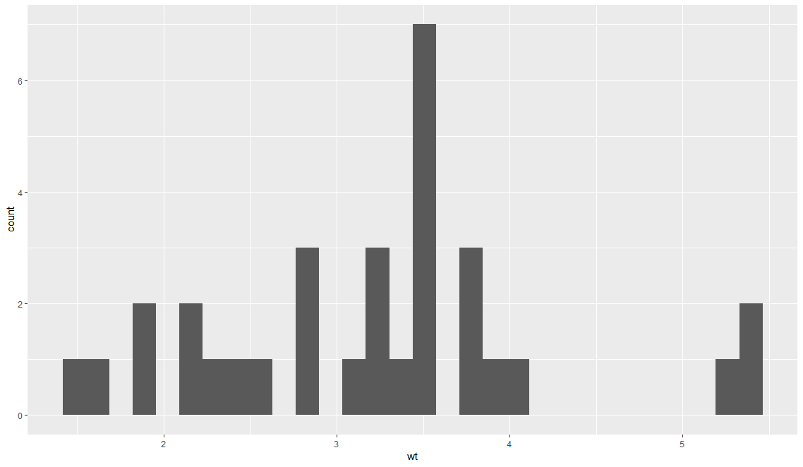
1
2ggplot(data=mtcars)+
geom_histogram(mapping=aes(x=wt))
可以明显看出,基础的R绘图的坐标轴在默认设置下连数据都难以囊括,因此这张图根本难以及格,而ggplot2不会出现这种问题。
画条形图的时候基础绘图系统也会出现类似问题:
基础绘图1
2counts <- table(diamonds$cut)
barplot(counts)
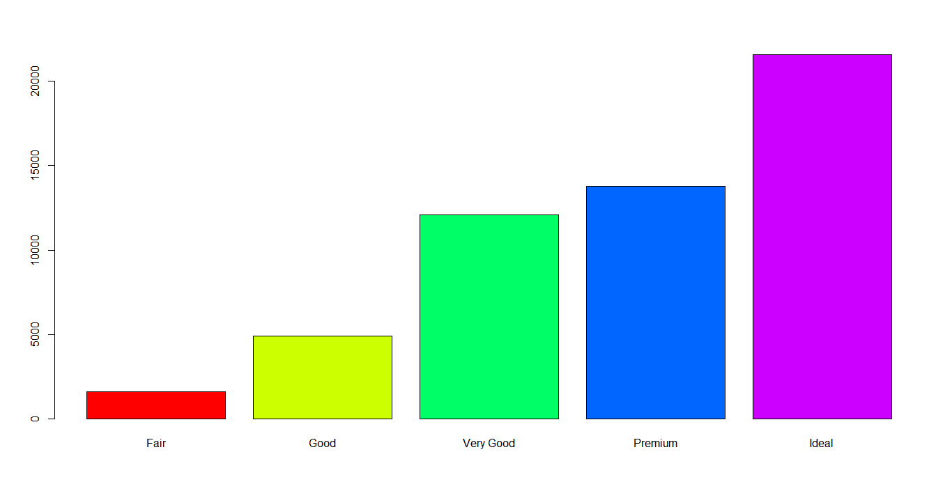
上图中坐标轴的长度比最长的部分还要短。
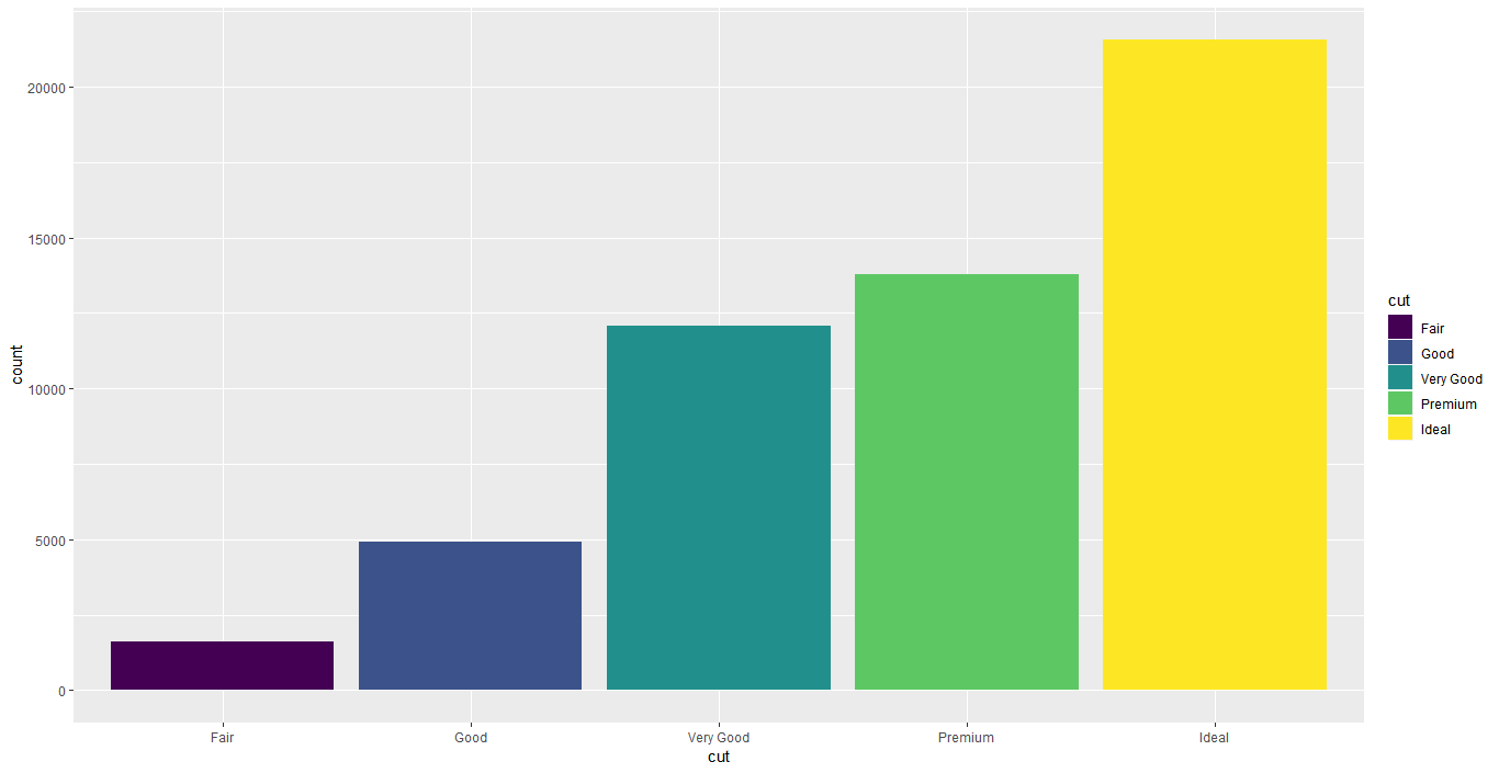
ggplot21
2ggplot(data=diamonds)+
geom_bar(mapping=aes(x=cut,y= ..count..,fill=cut))
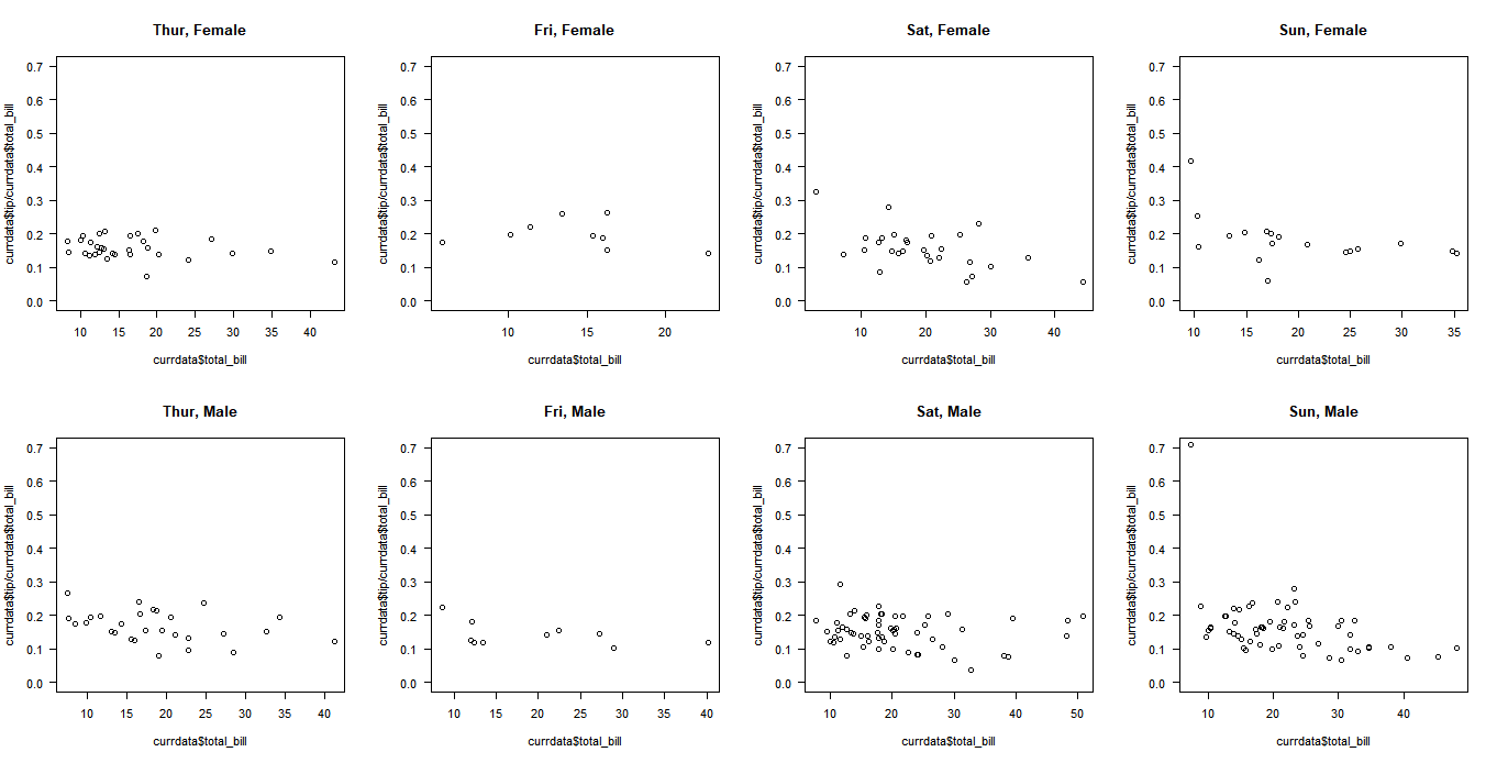
2.良好的分面设定ggplot2能够通过facet_grid()函数能够将数据依据不同的分类整齐划一地映射到不同的图形中,而基础绘图中要实现类似的功能需要使用循环,从这个角度来说,ggplot2能够起到四两拨千斤的作用(当然,ggplot2的四两拨千斤体现在很多方面,这只是一方面)。
基础绘图1
2
3
4
5
6
7
8
9
10
11library(reshape2)
par(mfrow=c(2,4))
days <- c("Thur", "Fri", "Sat", "Sun")
sexes <- unique(tips$sex)
for (i in 1:length(sexes)) {
for (j in 1:length(days)) {
currdata <- tips[tips$day == days[j] & tips$sex == sexes[i],]
plot(currdata$total_bill, currdata$tip/currdata$total_bill,
main=paste(days[j], sexes[i], sep=", "), ylim=c(0,0.7), las=1)
}
}
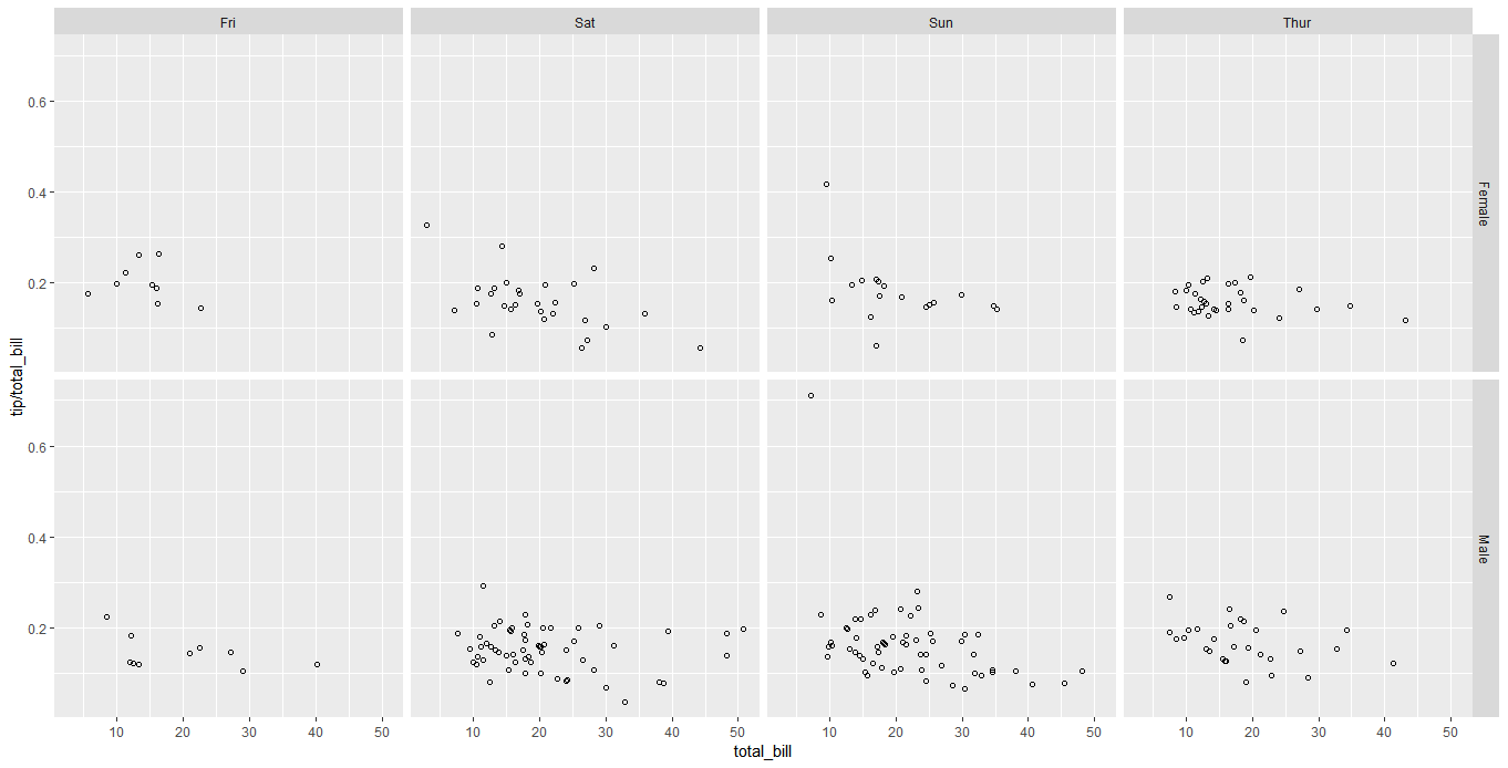
ggplot21
2
3library(reshape2)
sp <- ggplot(tips, aes(x=total_bill, y=tip/total_bill))+ geom_point(shape=1)
sp + facet_grid(sex ~ day)
3.方便使用的图层系统
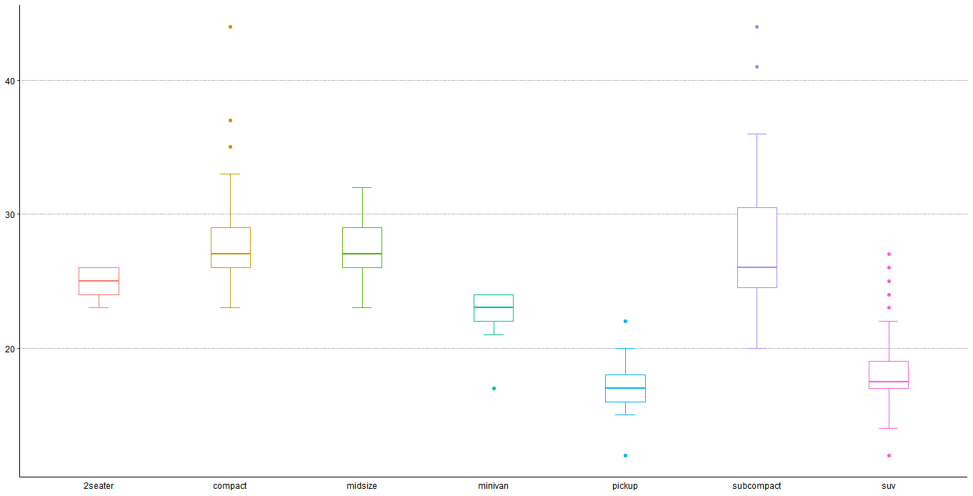
在画图过程中经常会进行多种图形的叠加,比方说散点图和线图的叠加,箱线图和抖动点图的叠加,ggplot2的图层系统使得在叠加过程中各个图层的坐标会进行自动调节和适应以达成整齐划一的效果,例如我想在箱线图的基础上增加抖动点图,先画出箱线图1
2
3
4
5
6
7
8
9
10
11
12
13
14
15library(ggplot2)
library(viridis)
p <- ggplot(data=mpg,mapping=aes(x=class,y=hwy))+
stat_boxplot(geom = "errorbar",width=0.15,mapping=aes(color=class))+
geom_boxplot(mapping=aes(color=class),width=0.3,position = "dodge2")+
theme_classic()+
theme(axis.ticks.x=element_blank())+
theme(axis.line=element_line(size=0.5))+
theme(legend.position ="None")+
#theme(plot.background = element_rect(fill="gray20"))+
theme(axis.title=element_blank())+
theme(axis.text = element_text(colour="black"))+
theme(plot.title = element_text(hjust=0.5))+
theme(panel.grid.major.y=element_line(color="grey",linetype = 6))
p
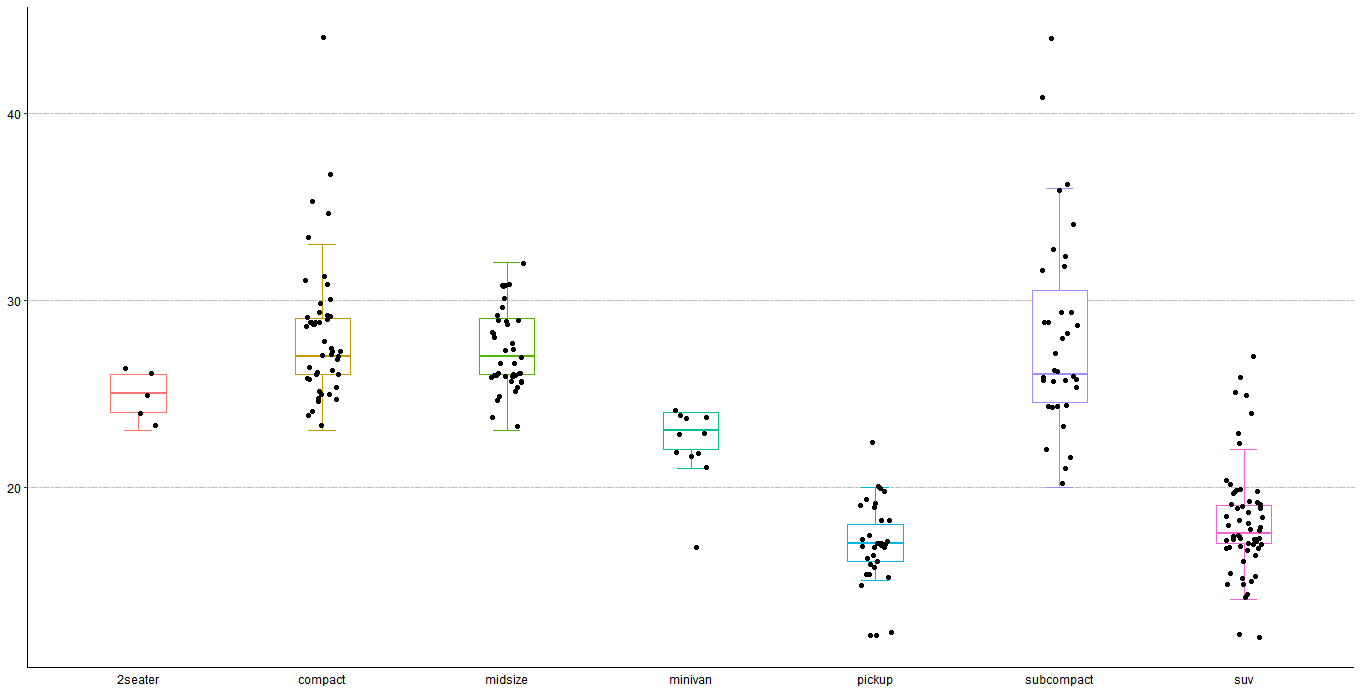
再在箱线图基础上增加抖动点1
2
3
4
5
6
7
8
9
10
11
12
13p <- ggplot(data=mpg,mapping=aes(x=class,y=hwy))+
stat_boxplot(geom = "errorbar",width=0.15,mapping=aes(color=class))+
geom_boxplot(mapping=aes(color=class),width=0.3,position = "dodge2",outlier.shape = NA)+
geom_jitter(width = 0.1)+
theme_classic()+
theme(axis.ticks.x=element_blank())+
theme(axis.line=element_line(size=0.5))+
theme(legend.position ="None")+
theme(axis.title=element_blank())+
theme(axis.text = element_text(colour="black"))+
theme(plot.title = element_text(hjust=0.5))+
theme(panel.grid.major.y=element_line(color="grey",linetype = 6))
p
4.强大实用的图形化语法
说到底,ggplot2区别于基础绘图系统的最大特点就在于其强大而实用的图形化语法,而这一特点也是以上所有ggplot2优点所存在的基础,图形化语法的存在,使得我们从数据本身以及图形本质来理解绘图,即
The grammar of graphics is based on the insight that you can uniquely describe any plot as a combination of a dataset, a geom, a set of mappings, a stat, a position adjustment, a coordinate system, and a faceting scheme.
图形化语法将任何一张图都看作是数据集、几何图形、映射关系、统计变换、位置设置、坐标系统以及分面系统的集合。
通过这一逻辑,可以总结出一个ggplot2的万能公式,从而使得我们只需要掌握很少的命令就能绘制大部分的图形1
2
3
4
5
6
7
8
9ggplot(data = <DATA>) +
<GEOM_FUNCTION>(
mapping = aes(<MAPPINGS>),
stat = <STAT>,
position = <POSITION>
) +
<COORDINATE_FUNCTION> +
<FACET_FUNCTION>+
<THEME_FUNCTION>
该公式与ggplot2图形的对应关系如下
| 命令 | 图形 |
|---|---|
| data = < DATA > | 数据集,例如上面的data=mpg |
| < GEOM_FUNCTION > | 几何对象,例如上面条形图的geom_bar |
| stat = < STAT > | 统计变换,例如上面条形图中的默认统计为stat=”count” |
| position = < POSITION > | 位置排列关系,例如上面箱线图的position = “dodge2” |
| < COORDINATE_FUNCTION > | 坐标轴相关的设置函数,例如coord_flip()用于交换坐标轴 |
| < FACET_FUNCTION > | 分面相关函数,例如上面的facet_grid(sex ~ day) |
| < THEME_FUNCTION > | 主题设置相关函数,例如theme_classic()+theme(axis.ticks.x=element_blank()) |
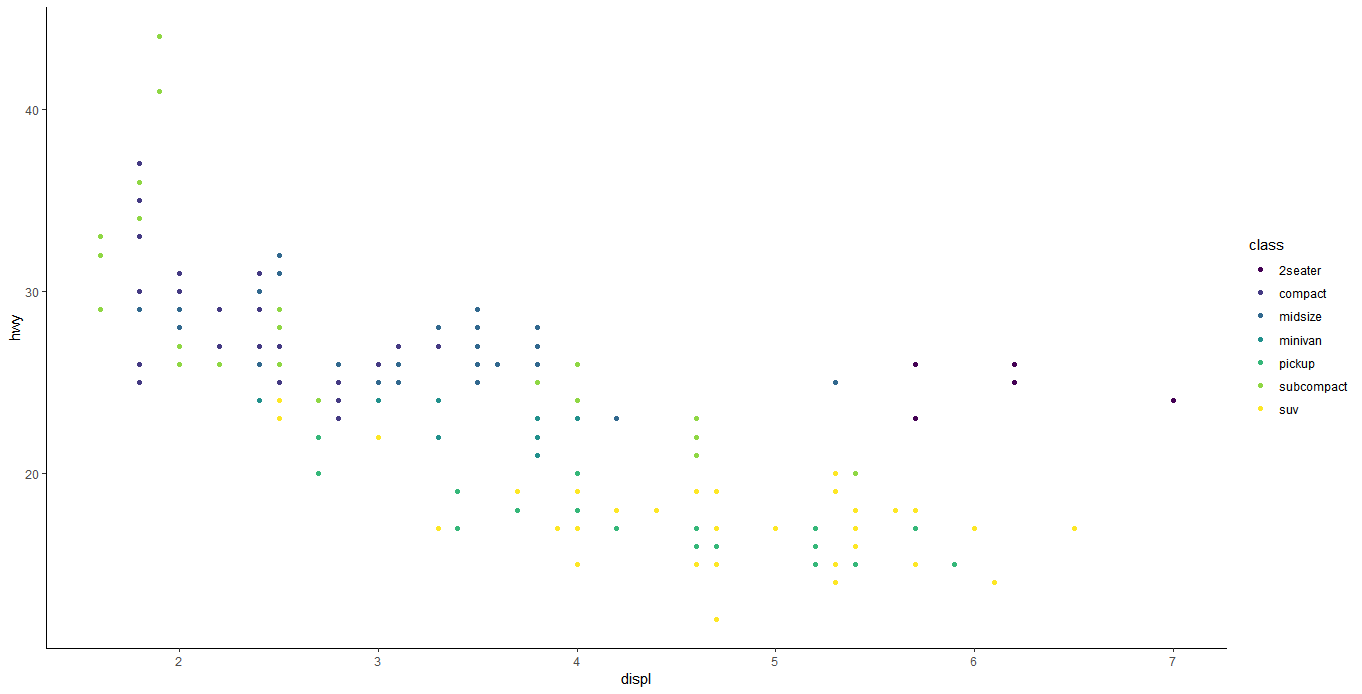
如果想画散点图:1
2
3
4ggplot(data = mpg) +
geom_point(mapping = aes(x = displ, y = hwy,color=class))+
theme_classic()+
scale_color_viridis(discrete=TRUE)
其对应关系为
| 命令 | 图形 |
|---|---|
| data = < DATA > | data = mpg |
| < GEOM_FUNCTION > | 几何对象,geom_point(mapping = aes(x = displ, y = hwy,color=class)) |
| stat = < STAT > | 默认统计为stat=”identity” |
| position = < POSITION > | 默认 |
| < COORDINATE_FUNCTION > | 无 |
| < FACET_FUNCTION > | 无 |
| < THEME_FUNCTION > | theme_classic()+scale_color_viridis(discrete=TRUE) |
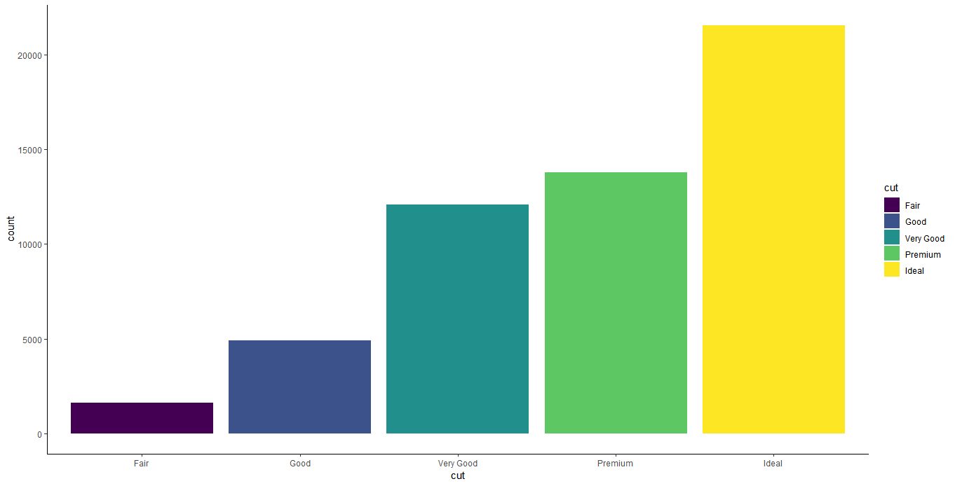
如果想画条形图:1
2
3ggplot(data = diamonds) +
geom_bar(mapping=aes(x=cut,fill=cut))+
theme_classic()
其对应关系为
| 命令 | 图形 |
|---|---|
| data = < DATA > | data = diamonds |
| < GEOM_FUNCTION > | geom_bar(mapping=aes(x=cut,fill=cut)) |
| stat = < STAT > | 默认stat=”count” |
| position = < POSITION > | 无 |
| < COORDINATE_FUNCTION > | 无 |
| < FACET_FUNCTION > | 无 |
| < THEME_FUNCTION > | theme_classic() |
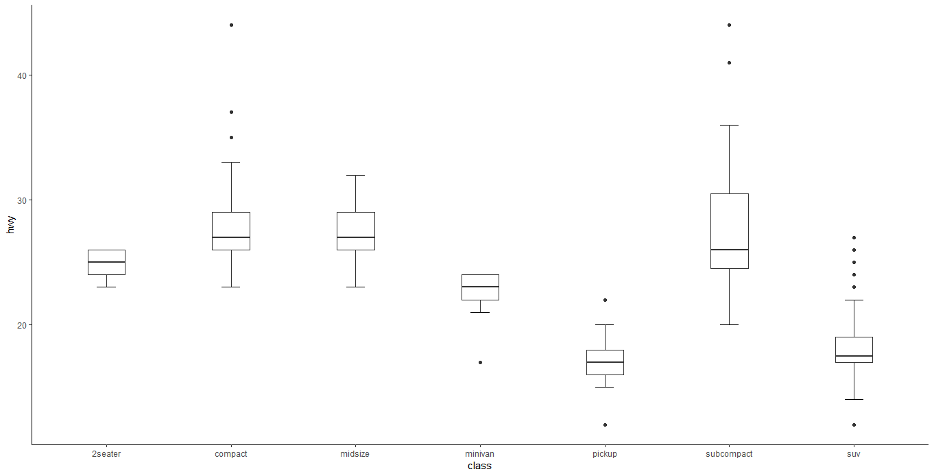
如果想画箱线图:1
2
3
4ggplot(data = mpg,mapping=aes(x=class,y=hwy)) +
stat_boxplot(geom = "errorbar",width=0.15)+
geom_boxplot(width=0.3)+
theme_classic()
对应关系为
| 命令 | 图形 |
|---|---|
| data = < DATA > | data = mpg |
| < GEOM_FUNCTION > | stat_boxplot(geom = “errorbar”,width=0.15) |
| stat = < STAT > | 默认stat=”identity” |
| position = < POSITION > | 无 |
| < COORDINATE_FUNCTION > | 无 |
| < FACET_FUNCTION > | 无 |
| < THEME_FUNCTION > | theme_classic() |
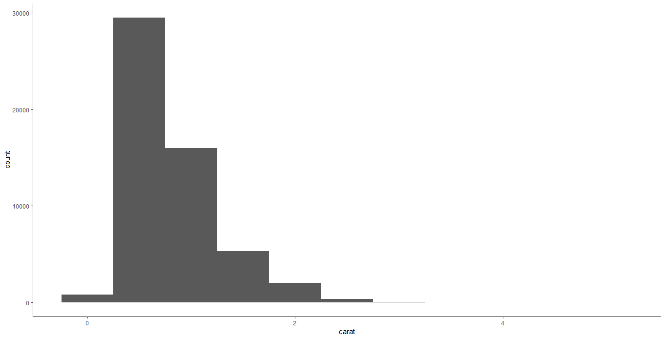
直方图1
2
3ggplot(data=diamonds)+
geom_histogram(mapping=aes(x=carat),binwidth=0.5)+
theme_classic()
对应关系
| 命令 | 图形 |
|---|---|
| data = < DATA > | data=diamonds |
| < GEOM_FUNCTION > | geom_histogram(mapping=aes(x=carat),binwidth=0.5) |
| stat = < STAT > | 默认stat=”count” |
| position = < POSITION > | 无 |
| < COORDINATE_FUNCTION > | 无 |
| < FACET_FUNCTION > | 无 |
| < THEME_FUNCTION > | theme_classic() |
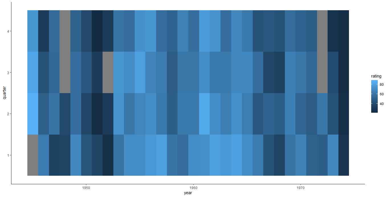
甚至于热图1
2
3
4
5
6
7
8
9pres_rating <- data.frame(
rating = as.numeric(presidents),
year = as.numeric(floor(time(presidents))),
quarter = as.numeric(cycle(presidents))
)
p <- ggplot(data=pres_rating, mapping=aes(x=year, y=quarter, fill=rating))+
geom_raster()+
theme_classic()
p
对应关系
| 命令 | 图形 |
|---|---|
| data = < DATA > | data=pres_rating |
| < GEOM_FUNCTION > | geom_raster() |
| stat = < STAT > | 默认stat=”identity” |
| position = < POSITION > | 无 |
| < COORDINATE_FUNCTION > | 无 |
| < FACET_FUNCTION > | 无 |
| < THEME_FUNCTION > | theme_classic() |
所有的这些绘图都可以用统一的语法格式概括到一起,当然每个图形都有一些细微的参数不太一样,但是这依然给我们带来了很多便利,提高了我们对于数据与图表对应关系的理解,方便了我们画不同的图形。
基本的图形元素及使用原则
坐标轴、轴须和坐标方格这些都属于导航元素(navigational elements), 这些导航元素提供了标准并帮助我们准确地获得长度以及比例的相关信息。这些元素在作图中需要保持以下原则:
1.总原则:必须与数据信息明显地区别开来,任何时候都要保持一个高 数据/墨水 比例,也就是说导航元素用尽可能少的墨水。下图fig 1a中由于没有将数据与线条区别开,导致读者很难快速从图中获得信息,而fig 1b则运用不同的颜色和透明度将数据与线条有效区分开,使人一目了然。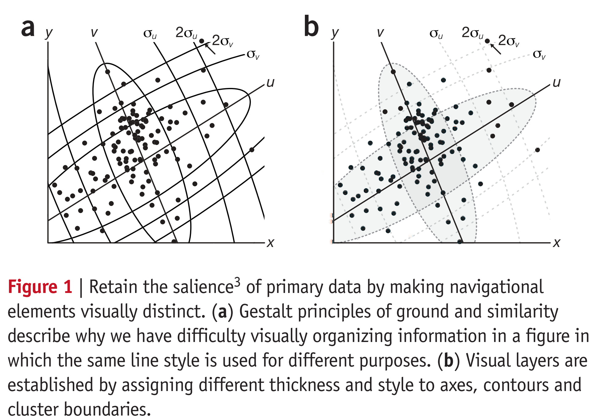
2.坐标轴
(1)坐标轴线条的宽度应当适度,0.5pt(像素点)就够了。(2)除非图片特别大,否则不能将坐标轴置于画布的边缘。(3)不要在坐标轴上加箭头,因为坐标轴的方向从来都不用怀疑。(4)多个图片一起放置时应该保持坐标轴刻度统一,因为在多图片比较时坐标轴范围的变化很容易被忽略,从而引起误导。如果想保持统一性,可以使用坐标中断(axis breaks),但是有些杂志不允许使用坐标中断,并且坐标中断很可能会掩饰一些很重要的pattern。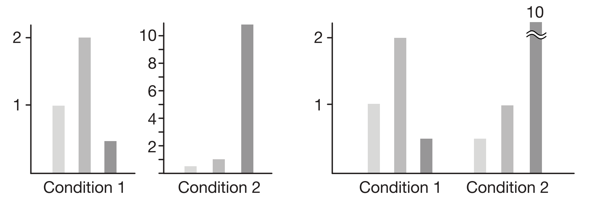
3.轴须:轴须要尽可能地少,因为如果轴须太多会增加图形的复杂性和认知负担。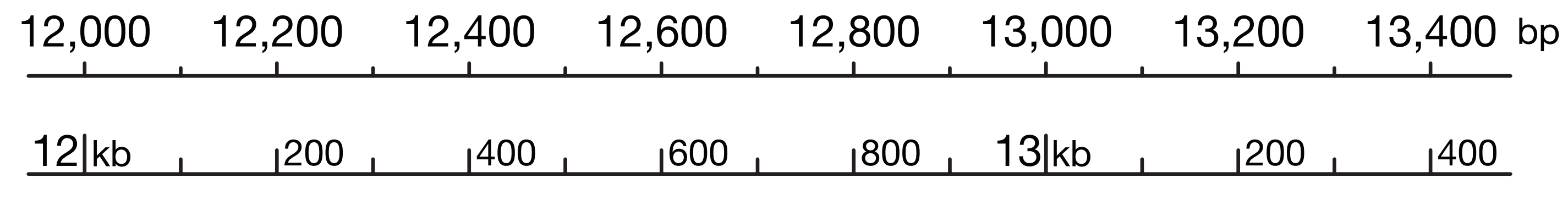
4.坐标方格:坐标方格的使用常常就是用浅色线条来用于比较比例和坐标轴轴须的相对位置。
(1)横线越多,读者就会越意识到数据的轻微波动。但是不要错误地使用坐标网格,因为坐标网格太密集会影响读者对数据的准确判断。总的来说,当你不知道怎么使用坐标网格时就不要使用它。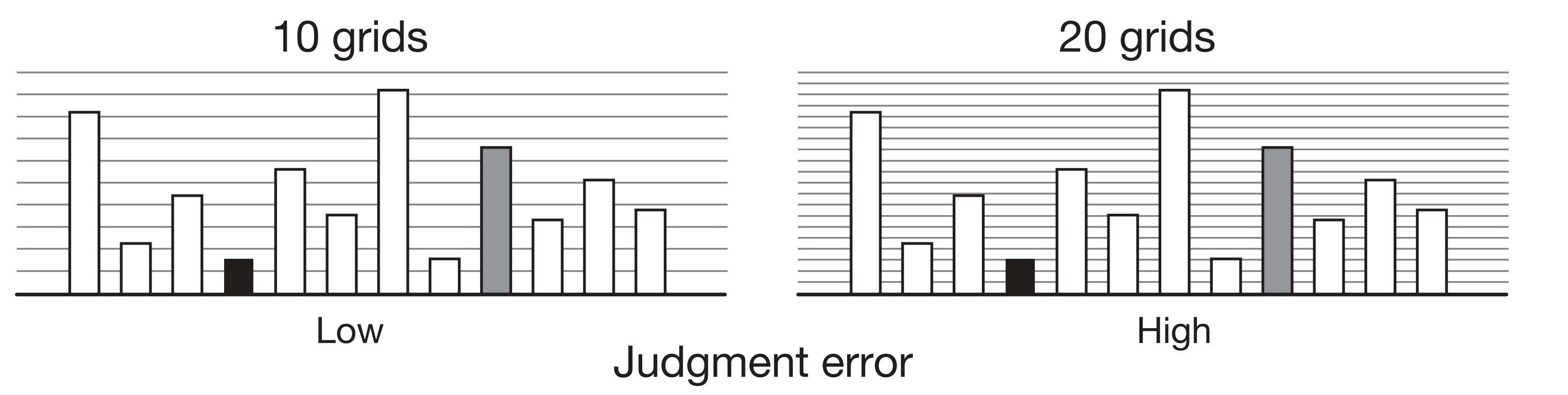
(2)坐标方格的颜色不能太深,否则会影响读者对数据的判断。建议网格不透明度在15%-45%之间,可以依数据密度来调整。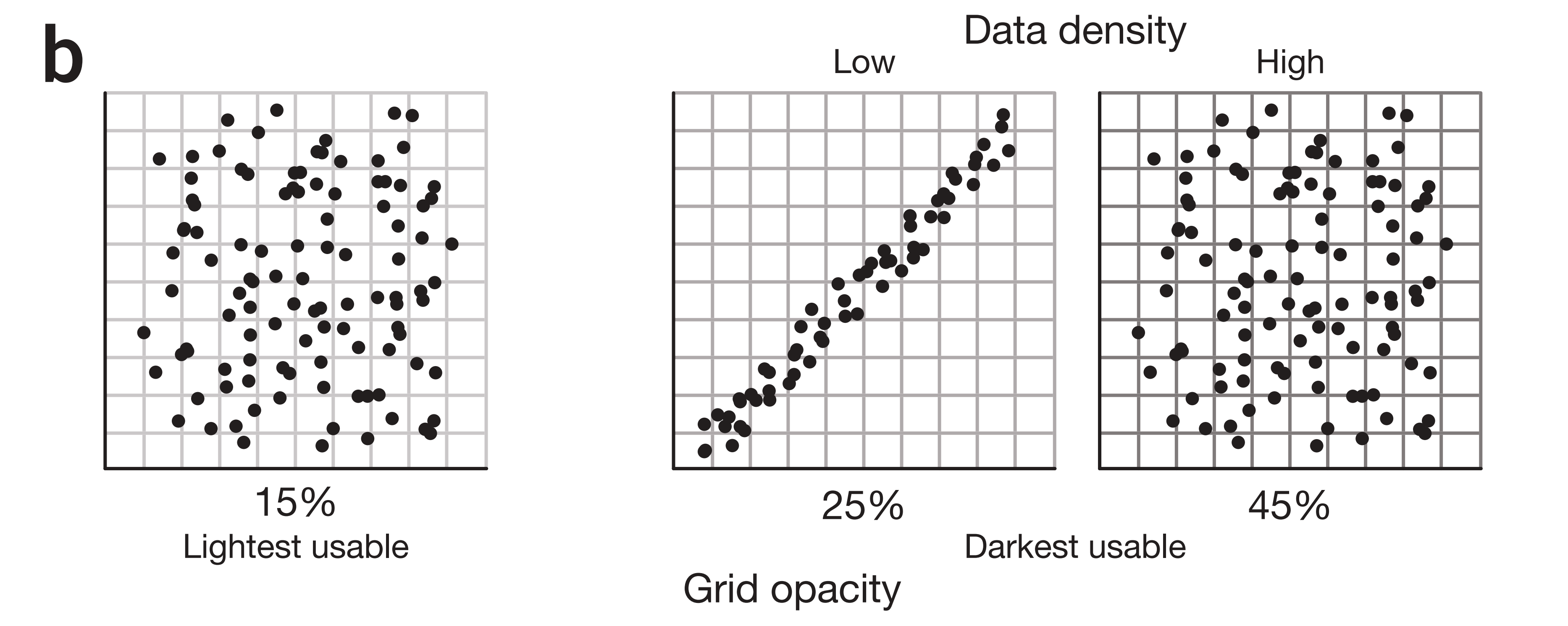
5.基本图形原则ggplot2的实现
下面就运用以上的原则来用ggplot2进行实践,比方说如果我想画一个条形图,
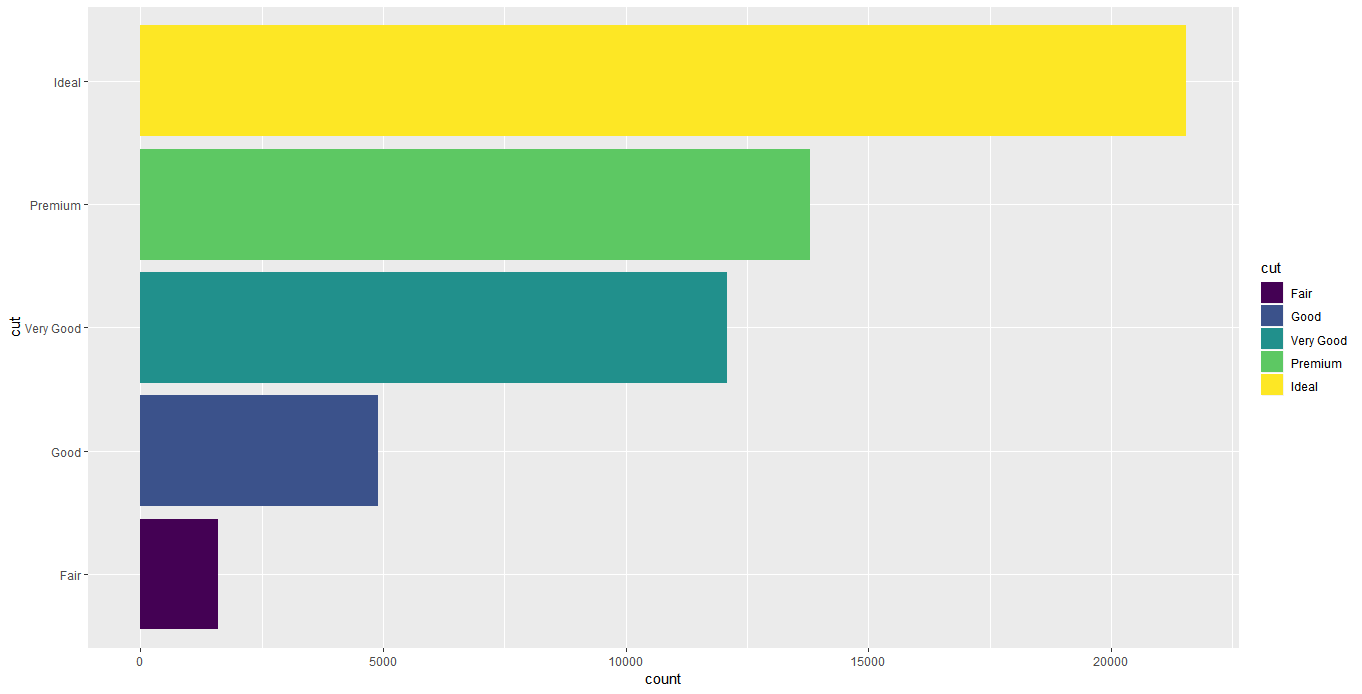
(1)一开始画图是这样的1
2
3ggplot(data=diamonds)+
geom_bar(mapping=aes(x=cut,y=..count..,fill=cut))+
coord_flip()
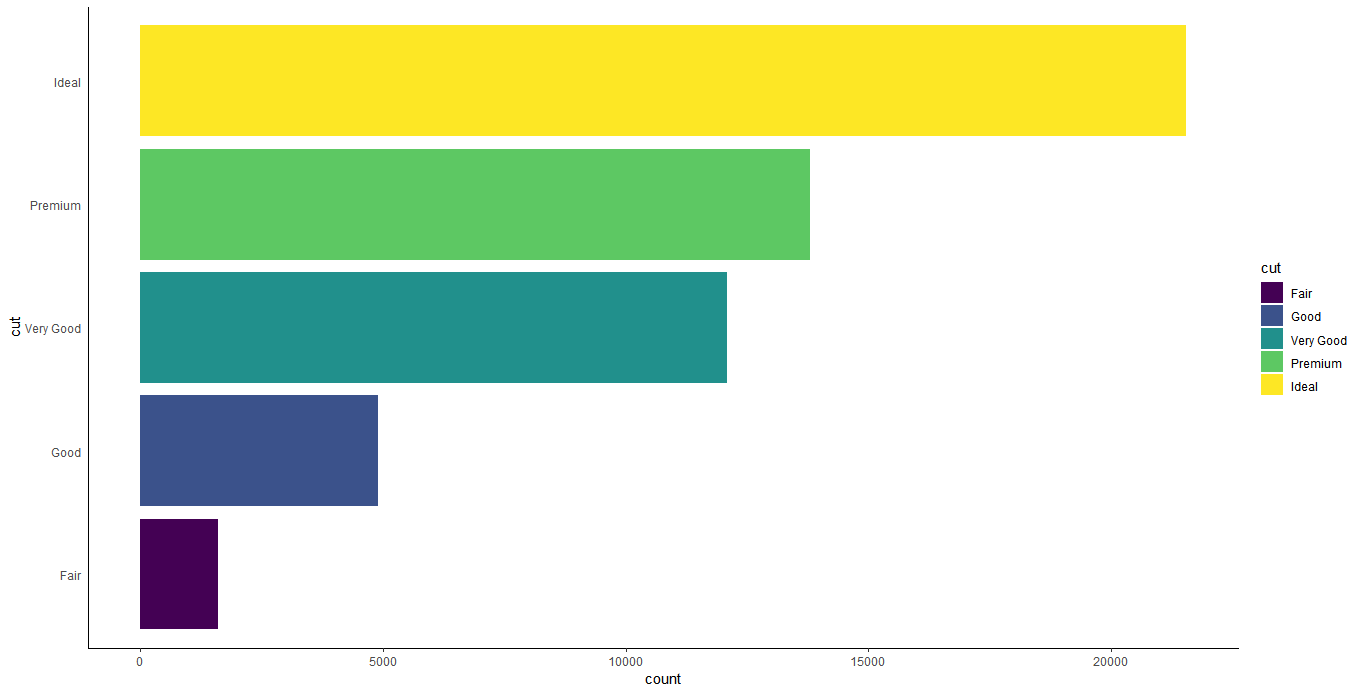
(2)很多人觉得ggplot2这个灰色背景太烂大街了,于是去掉1
2
3
4ggplot(data=diamonds)+
geom_bar(mapping=aes(x=cut,y=..count..,fill=cut))+
coord_flip()+
theme_classic()

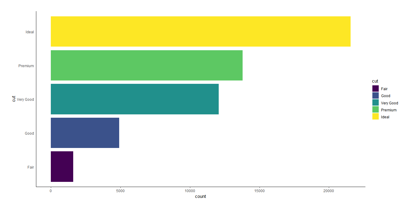
(3)前面说了,应该去除不必要的轴须,y轴的轴须就是不必要的:1
2
3
4
5ggplot(data=diamonds)+
geom_bar(mapping=aes(x=cut,y=..count..,fill=cut))+
coord_flip()+
theme_classic()+
theme(axis.ticks.y=element_blank())
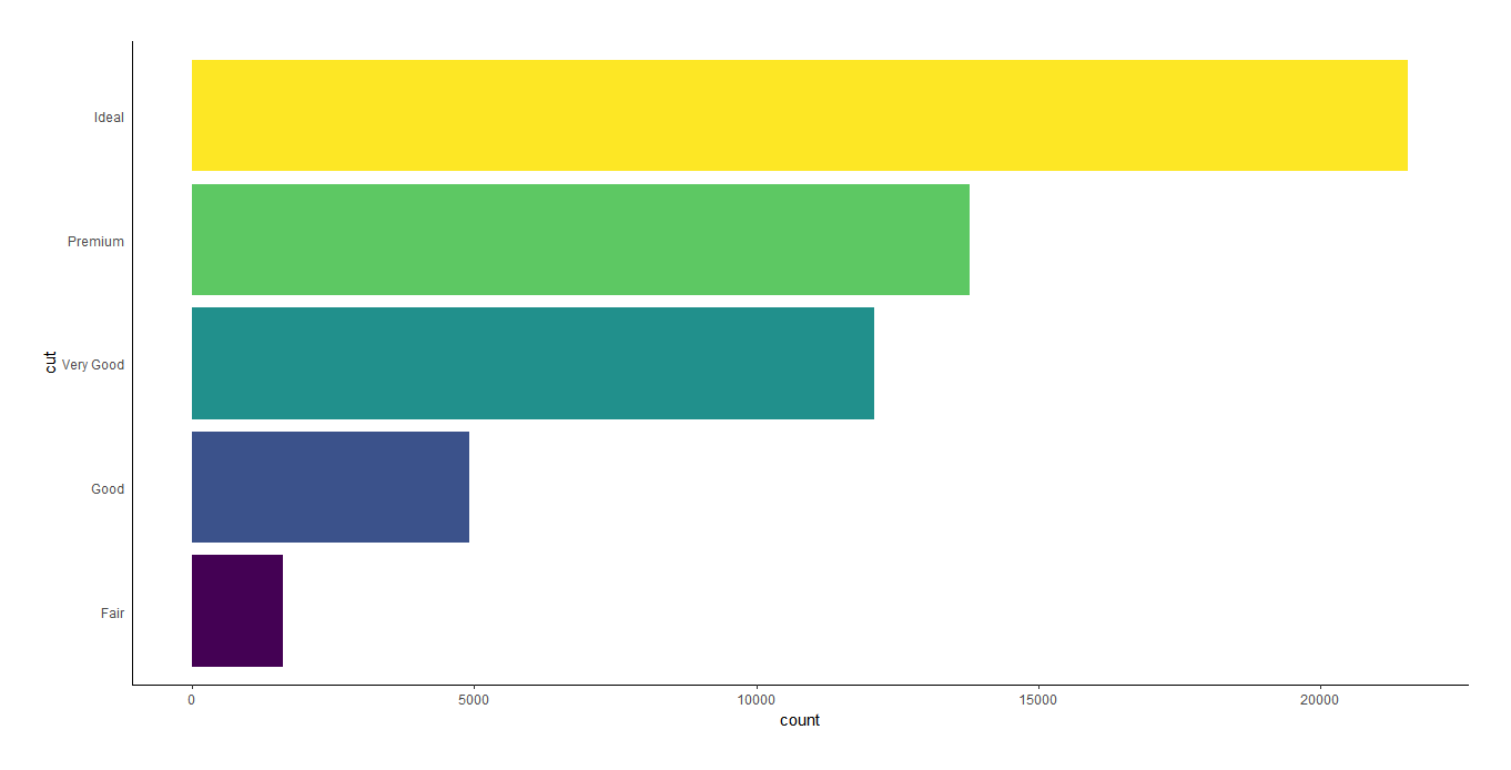
(4)坐标轴线的宽度设为0.51
2
3
4
5
6ggplot(data=diamonds)+
geom_bar(mapping=aes(x=cut,y=..count..,fill=cut))+
coord_flip()+
theme_classic()+
theme(axis.ticks.y=element_blank())+
theme(axis.line=element_line(size=0.5))

(5)调整边缘,使得图像不充满画布1
2
3
4
5
6
7ggplot(data=diamonds)+
geom_bar(mapping=aes(x=cut,y=..count..,fill=cut))+
coord_flip()+
theme_classic()+
theme(axis.ticks.y=element_blank())+
theme(axis.line=element_line(size=0.5))+
theme(plot.margin = margin(1,1,1,1,"cm"))
(6)由于图例与坐标轴纵轴表现的分类信息重复,因此我们要去除冗余信息,去掉图例1
2
3
4
5
6
7
8ggplot(data=diamonds)+
geom_bar(mapping=aes(x=cut,y=..count..,fill=cut))+
coord_flip()+
theme_classic()+
theme(axis.ticks.y=element_blank())+
theme(axis.line=element_line(size=0.5))+
theme(plot.margin = margin(1,1,1,1,"cm"))+
theme(legend.position = "None")
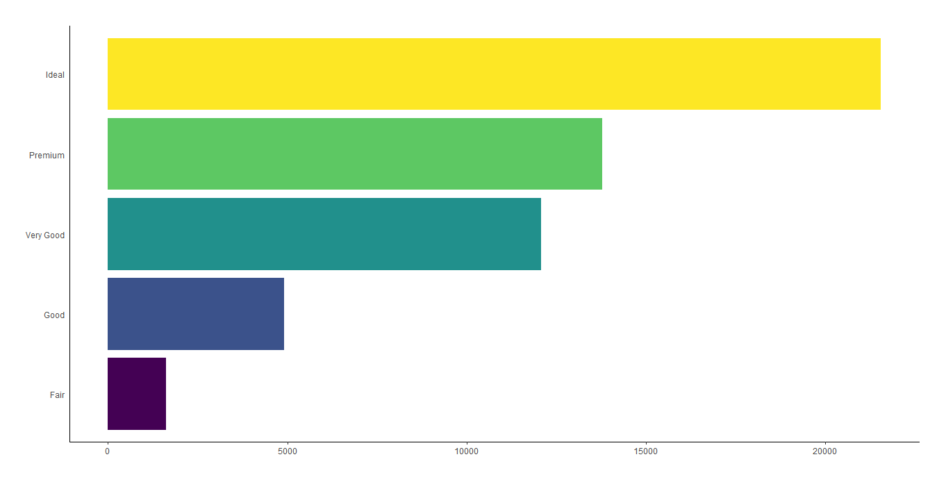
(7)x轴和y轴的标题看着也很碍眼1
2
3
4
5
6
7
8
9ggplot(data=diamonds)+
geom_bar(mapping=aes(x=cut,y=..count..,fill=cut))+
coord_flip()+
theme_classic()+
theme(axis.ticks.y=element_blank())+
theme(axis.line=element_line(size=0.5))+
theme(plot.margin = margin(1,1,1,1,"cm"))+
theme(legend.position = "None")+
theme(axis.title = element_blank())
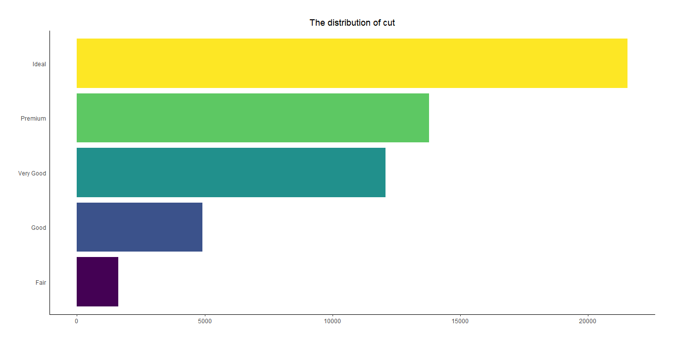
(8)向图中添加标题并使之居中1
2
3
4
5
6
7
8
9
10
11ggplot(data=diamonds)+
geom_bar(mapping=aes(x=cut,y=..count..,fill=cut))+
coord_flip()+
theme_classic()+
theme(axis.ticks.y=element_blank())+
theme(axis.line=element_line(size=0.5))+
theme(plot.margin = margin(1,1,1,1,"cm"))+
theme(legend.position = "None")+
theme(axis.title = element_blank())+
ggtitle("The distribution of cut")+
theme(plot.title = element_text(hjust=0.5))
(9)x轴和y轴的标签是灰色的,看着不太显眼1
2
3
4
5
6
7
8
9
10
11
12ggplot(data=diamonds)+
geom_bar(mapping=aes(x=cut,y=..count..,fill=cut))+
coord_flip()+
theme_classic()+
theme(axis.ticks.y=element_blank())+
theme(axis.line=element_line(size=0.5))+
theme(plot.margin = margin(1,1,1,1,"cm"))+
theme(legend.position = "None")+
theme(axis.title = element_blank())+
ggtitle("The distribution of cut")+
theme(plot.title = element_text(hjust=0.5))+
theme(axis.text = element_text(colour="black"))

(10)最后,添加网格线以便于查看数据分布情况1
2
3
4
5
6
7
8
9
10
11
12
13ggplot(data=diamonds)+
geom_bar(mapping=aes(x=cut,y=..count..,fill=cut))+
coord_flip()+
theme_classic()+
theme(axis.ticks.y=element_blank())+
theme(axis.line=element_line(size=0.5))+
theme(plot.margin = margin(1,1,1,1,"cm"))+
theme(legend.position = "None")+
theme(axis.title = element_blank())+
ggtitle("The distribution of cut")+
theme(plot.title = element_text(hjust=0.5))+
theme(axis.text = element_text(colour="black"))+
theme(panel.grid.major.x=element_line(color="grey",linetype = 6))

参考资料
1.Schwartz, Daniel L., Jessica M. Tsang, and Kristen P. Blair. The ABCs of how we learn: 26 scientifically proven approaches, how they work, and when to use them. WW Norton & Company, 2016.
2.Moore, David S., William I. Notz, and William Notz. Statistics: Concepts and controversies. Macmillan, 2009.
3.Why we love these 5 data visualization tools: https://www.softwebsolutions.com/resources/five-data-visualization-tools.html
4.Why use ggplot2:https://github.com/tidyverse/ggplot2/wiki/Why-use-ggplot2
5.Comparing ggplot2 and R Base Graphics : https://flowingdata.com/2016/03/22/comparing-ggplot2-and-r-base-graphics/
6.Wickham, H. and G. Grolemund (2016). R for Data Science: Import, Tidy, Transform, Visualize, and Model Data, O’Reilly Media.
7.Krzywinski, M. (2013). “Axes, ticks and grids.” Nature methods 10: 183.